Logistic Regression

View the Data:

Data transformations and modeling:

library(grid) # Grob()
library(ggplot2) # ggplot()
donner = read.table("donner.txt")
colnames(donner) = c("age","sex","survive")
# Age
# Sex: (1=male, 0=female)
# Survive (1=survived, 0=dead)
age = donner$age
sex = donner$sex
survive = donner$survive


# Logistic Regression Model: Survival as a function of age, sex, and the interaction
model.c = glm(survive~age*sex,family=binomial("logit"))

# Data by Sex
donner.cM = data.frame(age[which(sex==1)],model.c$fitted.values[which(sex==1)])
donner.cF = data.frame(age[which(sex==0)],model.c$fitted.values[which(sex==0)])
text.xaxis = textGrob(label="Note: Data is jittered to see all values.",
                      gp=gpar(cex=0.75,fontface="italic"))

# Logistic Regression Functions
donner.male.int.fun <- function(x) {
  exp(7.24638-(0.19407*x)-6.92805+(0.16160*x))/
    (1+exp(7.24638-(0.19407*x)-6.92805+(0.16160*x)))
}
donner.female.int.fun <- function(x) {
  exp(7.24638-(0.19407*x))/(1+exp(7.24638-(0.19407*x)))
}

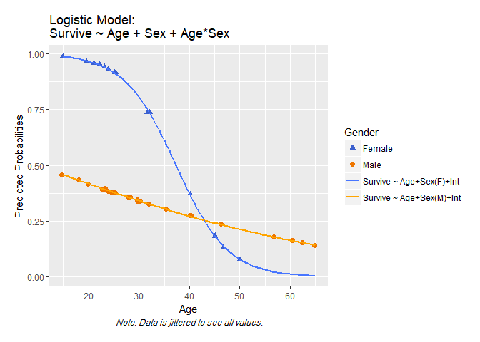
Logistic Regression Plot with Interaction

plot.donnerc = ggplot() +
  geom_jitter(data=donner.cM,mapping=aes(x=donner.cM[,1],y=donner.cM[,2],color="Male"),
              size=2,shape=16) +
  geom_jitter(data=donner.cF,mapping=aes(x=donner.cF[,1],y=donner.cF[,2],color="Female"),
              size=2,shape=17) +
  theme(plot.margin=unit(c(1,1,2,1),"lines")) +
  annotation_custom(grob=text.xaxis,xmin=40,xmax=40,ymin=-0.2,ymax=-0.2) +
  stat_function(mapping=aes(color="Survive ~ Age+Sex(M)+Int"),fun=donner.male.int.fun,size=1) +
  stat_function(mapping=aes(color="Survive ~ Age+Sex(F)+Int"),fun=donner.female.int.fun,size=1) +
  scale_colour_manual(name="Gender",
                      values=c("Male"="darkorange2",
                               "Female"="royalblue3",
                               "Survive ~ Age+Sex(M)+Int"="orange",
                               "Survive ~ Age+Sex(F)+Int"="royalblue1")) +
  guides(colour=guide_legend(override.aes=list(linetype=c(0,0,1,1),
                                               shape=c(17,16,NA,NA))),
         guide="legend") +
  labs(title="Logistic Model:\nSurvive ~ Age + Sex + Age*Sex",
       x="Age",y="Predicted Probabilities")
plot.c = ggplot_gtable(ggplot_build(plot.donnerc))
plot.c$layout$clip[plot.c$layout$name=="panel"] <- "off"
grid.draw(plot.c)